
A first look at a real mine, and a surface that misleads
Today in short
- I moved from small generated mines to newman1, a real mine from the public MineLib library, with published best-known results to check against.
- Grade means something different here. It’s grams of gold per tonne of rock, not the share of a block that is ore. A block goes wholly to the mill or wholly to waste.
- The dataset can’t satisfy all of my model’s rules. Capacities, precedence and “mine before you process” carry over. Stockpiling, splitting a block across periods and grade blending don’t.
- I use newman1 only as a mine. My model keeps its own rules, and MineLib’s published results are for reference, not targets.
- First runs. Full MILP 22,386,899, greedy 21,800,955, blind 4,243,334.
- Blind stalls on this mine. It can’t see the ore under the waste, so it stops digging early.
- newman1 is shelved for now. Later it will be placed in a full cube and scaled down by merging blocks into small, medium and large instances.
- A misleading surface makes drilling shine. On a small mine where the surface is richer on one side and the ore underneath is richer on the other, every shaft gets within 2.5% of perfect information for under 100 of drilling, greedy falls 40% behind, and the minimum mining rule barely matters.
Why a real dataset
Small generated mines are good for understanding why a method behaves the way it does, but they’re easy to tune without meaning to. A public benchmark gives a fixed, realistic test that other researchers have already solved, so my results can be compared directly with theirs.
MineLib is a standard library of open-pit mining problems, and newman1 is one of its smaller instances. Source pages: MineLib datasets and newman1.
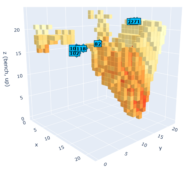
The mine at a glance
| Blocks | 1,060 |
| Shape | Irregular pit inside a 22 × 22 × 24 grid, filling only 9.1% of that box |
| Precedence | Each block needs up to 5 blocks on the bench above it removed first (3,922 links) |
| Periods | 6, with an 8% discount rate |
| Mining limit per period | 2,000,000 t |
| Processing limit per period | 1,100,000 t |
| Minimum mining | None |
| Grade blending limits | None |
| Total rock | 5.62 Mt, about 2.8 periods of mining |
Blocks don’t all weigh the same. Most full blocks weigh 5,664 t. Full oxide ore blocks weigh 5,184 t because oxide rock is lighter. 182 blocks are partial (from 74 t up), mostly where the ground surface cuts through the top of a column. My code already uses each block’s own weight.
The gaps aren’t holes. Every (x, y) column is a solid stack. The gaps in the picture are just columns that start lower down, so the space above them is air. The model only knows the 1,060 real blocks. One side effect is that near the pit edges some slope links point to rock MineLib left out of the instance, so the wall slopes there are only approximate. That’s a property of the dataset, not my code. In the blind setting, the scheduler starts by seeing the top block of each of the 170 columns.
What “grade” means here
In my generated mines, grade was the share of a block that is ore (0 to 1), and only that share was processed. In newman1, grade is grams of gold per tonne of rock, which is why values go up to 3.7. MineLib doesn’t name the metal, but it fits. The price term of 19.29 per gram works out to $600 per troy ounce.
Each block is sent wholly to the mill or wholly to waste. Its processing value is
(19.29 × recovery × grade − processing cost) × tonnage
with different costs and recoveries for oxide ore (cheaper to process, better recovery) and fresh rock. That gives a break-even (cutoff) grade.
| Rock | Cutoff grade |
|---|---|
| Fresh rock (FROR, FRWS) | about 1.04 g/t |
| Oxide ore (OXOR) | about 0.47 g/t |
So a block can contain some gold and still be waste. Block 115, for example, is fresh rock at 0.76 g/t, below its cutoff. The 91 blocks of type “0” have zero grade and are treated as plain waste.
Because the value follows a formula, hidden blocks can be re-valued from an estimated grade, which is exactly what the blind and partial (drilling) schedulers need.
Where my model and newman1 don’t match
| Rule | My model | newman1 (MineLib) |
|---|---|---|
| Mining and processing limits | ✓ | ✓ same |
| Precedence (blocks above first) | ✓ | ✓ same |
| Process only what’s been mined | ✓ | ✓ same |
| When ore is processed | Any later period (a free stockpile) | Same period it’s mined |
| Mining a block | Can be split across periods | All in one period |
| Grade blending limits | Optional | None |
| Minimum mining | Optional | None |
The last four rows mean my model is a little looser than MineLib’s, so its NPV can come out slightly higher than their published values.
Decision. I use newman1 only as a mine, meaning its blocks, values, slopes and capacities. My thesis model stays as it is, with blocks that can be mined over several periods and ore that can be processed later. MineLib’s published results follow different rules, so they’re kept for reference only and are not targets to match.
Technical detail. Fitting newman1 into the code
- Loader
cleaned/newman1_loader.pyreads the MineLib files into theMineclass. It reproduces the ultimate pit value (26,086,899) exactly. - My code discounts from period 1, MineLib from period 0, so my NPV = MineLib value ÷ 1.08. I confirmed this by solving MineLib’s LP relaxation, which reproduces their published bound exactly.
- The big-M in constraint 1 was 1e6, too small for this mine. It needs at least 5.62e6.
newman1_compare.pyruns the full MILP, blind and greedy, and checks every schedule against my constraints.- Ore rule. A block is ore when its processing value beats its mining value, which gives 572 ore blocks (3.02 Mt).
First results
My NPVs below use my own discounting (from period 1).
| Method | NPV |
|---|---|
| Full MILP | 22,386,899 |
| Greedy | 21,800,955 |
| Blind | 4,243,334 |
The full MILP solved in 14 seconds. Greedy gets within about 3% of it. Blind collapses to less than a fifth.
For reference against MineLib. Converted to MineLib’s discounting, my full MILP is 24,177,851, about 2% above their best listed schedule (23,658,230) and still below their upper bound (24,486,549). That’s expected, partly because my model is looser, and MineLib’s listed value comes from an older heuristic. Only 2 blocks were actually split across periods and no ore was held over, so most of the difference is just a better schedule. Since MineLib’s rules aren’t targets, I don’t need to match their number.
What each method does in period 1
| Blocks mined | Shared with full MILP | Average ore grade | |
|---|---|---|---|
| Full MILP | 407 | 1.59 g/t | |
| Greedy | 420 | 325 | 1.31 g/t |
| Blind | 153 (only 18 waste) | 134 | 1.38 g/t |
- Full MILP digs the full 2 Mt, 196 ore blocks and 211 waste blocks. Every waste block sits above ore it processes in periods 1 and 2. Block 271, for example, is worthless rock on the top bench, but 133 ore blocks of 1.5 to 2 g/t lie under it. The MILP pays to strip it now so the rich ore reaches the mill early.
- Greedy grabs the best block on offer each step, starting with blocks 103 and 102 (2.0 and 2.9 g/t), which have little on top. It strips waste only when nothing better is available, so its period-1 ore is lower grade.
- Blind sees only the top of each column. Blocks 82 and 118 sit low on the side of the pit and look profitable, but block 118 barely beats its cutoff. Blind can’t justify stripping a block like 271, because it can’t see the ore underneath. So it stops after 679,000 t in period 1 and never sees 785 of the blocks. That’s the same stall as on my generated decoy mines.
The order of actions inside a period doesn’t affect NPV. Everything in a period is discounted the same, and the replay simply does all digging first, largest blocks first.
Back on the small mine. A surface that misleads
The last run of the day went back to the 4 × 5 × 4 mine (10 t blocks, 7 periods, my usual capacities) with a new grade layout built to test the shaft idea cleanly. The surface points one way and the ore underneath points the other.
- Surface. Richest at the far corner (row 4, column 3), poorest at the near corner (row 0, column 0), but nowhere pure waste. It stays below 0.5, so surface ore can’t fill the 40 t plant on its own. Only the two far-corner blocks (0.40 and 0.45) reach the 0.4 cutoff alone. The rest can only be processed blended with richer ore.
- Layers 1 and 2. The reverse. Richest under the near corner (up to 1.00), poorest under the far one.
- Layer 3. Waste.
Surface (layer 0)              Layer 1
richer toward far corner       richer toward near corner
 0.05 0.12 0.18 0.25            1.00 0.87 0.73 0.60
 0.10 0.17 0.23 0.30            0.90 0.77 0.63 0.50
 0.15 0.22 0.28 0.35            0.80 0.67 0.53 0.40
 0.20 0.27 0.33 0.40            0.70 0.57 0.43 0.30
 0.25 0.32 0.38 0.45            0.60 0.47 0.33 0.20
All three shafts start on the poor side of the surface, so they sample the rich ore underneath. Earlier versions with a richer surface made every shaft worthless, because the surface ore alone already filled the plant. The parameters are saved as cleaned/runs/params_4x5x4_opposite_p7.yaml.
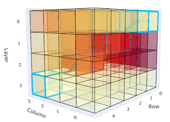
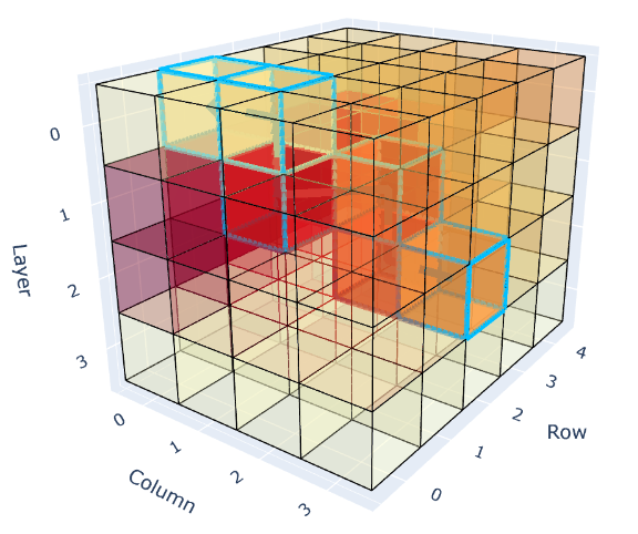
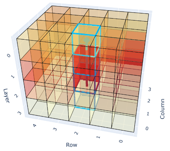
Results
| NPV | Blind | Diagonal | Shallow | Vertical | Full information | Greedy |
|---|---|---|---|---|---|---|
| No minimum | 891 | 12,589 | 12,482 | 12,589 | 12,675 | 8,874 |
| Net of drill cost | 12,497 | 12,416 | 12,543 | |||
| 20 t minimum | 8,641 | 12,582 | 12,559 | 12,362 | 12,675 | 8,874 |
| Net of drill cost | 12,490 | 12,493 | 12,316 |
Drill costs are 92 (diagonal), 66 (shallow) and 46 (vertical).
1. The minimum no longer distorts partial. With and without the 20 t minimum, partial changes by at most 1.8% (vertical), and diagonal barely moves (12,589 against 12,582). On the lens layout the minimum cost partial up to 20%. The difference is that this surface has some value, especially blended with the rich ore below, so the planner never sees its future periods as forced waste mining and has no reason to ration its stripping.
2. Every shaft gets partial close to perfect information. Partial lands within 2.5% of full information in every case. With no minimum each shaft gains about 11,600 over blind for under 100 of drilling. With the minimum the gain is about 3,700 to 3,900, because blind digs further on its own when forced to.
3. All three shafts are nearly equal. The rich zone is broad, not a small lens, so any shaft that hits it is enough. Net of cost, the cheapest shaft wins with no minimum (vertical, 12,543), and diagonal and shallow tie with the minimum. Differences of a few hundred are within the near-tie noise seen before.
4. Greedy falls far behind (8,874). It takes whatever looks best right now, which is the richer far side of the surface. That’s exactly the trap this layout sets, because the real ore is under the other side. Partial beats greedy by about 40%.
5. Blind with no minimum stops almost at once (891). It mines the two processable surface blocks at the far corner, finds poor ore below them, and stops. With the minimum it’s forced to keep digging and reaches part of the rich zone (8,641).
Why vertical works here but failed on the lens
The vertical shaft goes straight down through blocks 10, 30, 50 and 70 (row 2, column 1).
| Layer | Block | Grade |
|---|---|---|
| 0 (surface) | 10 | 0.22 |
| 1 | 30 | 0.67 |
| 2 | 50 | 0.72 |
| 3 | 70 | 0 |
It starts on the poor side and finds good ore one layer down, under blocks the scheduler can already see.
- Stripping is cheaper. On the lens, the 9 surface blocks above vertical’s ore were pure waste, so clearing them for one rich block only broke even and the MILP never started. Here those blocks grade 0.10 to 0.33. They carry some ore that can be processed blended with the richer ore below, so stripping partly pays for itself.
- The rich zone is broad. Once digging starts at row 2, column 1, every block uncovered nearby is good, and each reveal leads the scheduler toward the richest corner. That’s why vertical with no minimum ends with exactly the same NPV as diagonal (12,588.60). Once digging starts on the near side, the rest of the schedule is the same, and vertical is the cheapest shaft.
How these runs plan
All periods at once, with re-planning. Each solve plans the whole remaining horizon (from now to period 7) as one MILP, with the 20 t minimum on every period of the plan. The loop carries out one action, reveals any newly exposed blocks, and solves the whole remaining horizon again. So every decision comes from a full multi-period plan, redone as new blocks appear. This is the method I settled on yesterday, and it’s part of why these results improved.
The full-information value (12,675) is the one-shot MILP. It knows every grade and solves all 7 periods once, with no re-planning.
What this means for the thesis
This layout gives the clearest support for the shaft approach. When the surface misleads about what’s below, one cheap shaft through the poor-looking side recovers almost all the value of perfect information. It works with and without a minimum, and it avoids the waste-rationing problem. The lens layout is the counter-case. When the surface over the ore is pure waste and a minimum applies, the same method rations its stripping.
Plan. newman1 is shelved for now
newman1 is on hold until the rest of the framework is complete. When I come back to it, the plan is as follows.
- Place the mine in a full cube. A real mine sits inside solid ground, so the irregular pit will be put into a complete rectangular block model, with the empty cells filled in as blocks. This matches how my own code represents a mine, and it also fixes the approximate pit walls, since the rock MineLib left out will now exist.
- Shrink it by combining blocks. Filling the cube increases the block count a lot, so the problem will be scaled down by merging neighbouring blocks into larger ones. That gives three sizes of the same mine.
| Instance | How it’s built |
|---|---|
| Small | Combine each group of 4 neighbouring blocks into one |
| Medium | Combine each pair of neighbouring blocks into one |
| Large | The full cube, with no merging |
This gives one real mine at three sizes, so I can see how each method (MILP, greedy, blind, partial and Sim + LLM) holds up as the problem grows.
Next
When newman1 comes back
- Place newman1 in a full cube and build the small, medium and large instances by merging blocks.
- Get blind past the stall, with a minimum mining rule or a larger reveal bonus.
- Adapt the partial (drilling) code. It finds “the block underneath” by ID arithmetic, which only works on a full grid (the cube will help here), and estimated blocks need the newman1 value formula.
- Add exploratory shafts and run partial on all three sizes.